
dplyrでデータ加工入門【filter・select・mutate・group_by・summarise】
 酒井 裕麻株式会社Bistro 代表取締役社長
Rでデータを読み込んだら、次は「必要な行だけに絞る」「店舗ごとに合計する」といったデータ加工です。こうした作業を、Excelよりずっと速く、しかも手順を残しながら行えるのが dplyr(ディープライヤー) パッケージです。
この記事では、dplyrの基本となる5つの関数とパイプ(%>%)の使い方を、実際の売上データを使って解説します。最後には、集計した結果をグラフにするところまで進みます。
参考記事
RでCSVの文字化けを直す方法とExcelファイルの読み込み【実行結果付き】
Rのパッケージのインストール方法と読み込み方【よくあるエラーの対処法付き】
この記事で使うデータ
架空の店舗の売上データ sales.csv を使います。2026年1〜3月の、3店舗(新宿・渋谷・横浜)×3カテゴリ(食品・飲料・日用品)の日別データです。
| 列名 | 内容 |
|---|---|
| date | 日付 |
| store | 店舗 |
| category | カテゴリ |
| customers | 客数 |
| sales | 売上(円) |
| ad_spend | 広告費(円) |
install.packages("dplyr")  # 最初の1回だけ
library(dplyr)
sales <- read.csv("sales.csv")
dplyrの5つの基本関数
| 関数 | やること | Excelでいうと |
|---|---|---|
filter() |
条件に合う行を絞り込む | フィルター |
select() |
必要な列を選ぶ | 列の削除・並べ替え |
mutate() |
新しい列を追加する | 計算列の追加 |
arrange() |
並び替える | 並べ替え |
group_by() + summarise() |
グループごとに集計する | ピボットテーブル |
パイプ(%>%)で処理をつなぐ
dplyrでは、処理を %>%(パイプ)でつないで書きます。「左のデータを、右の処理に渡す」という意味で、「〜して、それから〜する」と上から順に読めるのが特徴です。
sales %>% filter(store == "渋谷店") %>% head(3)これは「salesから、渋谷店の行だけを絞り込んで、先頭3行を表示する」という意味です。
※%>% は Ctrl + Shift + M(Macは Cmd + Shift + M)で入力できます。R 4.1以降では、標準の |> も同じように使えます。
filter():行を絞り込む
sales %>% filter(store == "渋谷店") %>% head(3)実行結果
        date  store category customers  sales ad_spend
1 2026-01-01 渋谷店   日用品        63  60030    17000
2 2026-01-01 渋谷店     食品       121 167150    27000
3 2026-01-01 渋谷店 飲料 69 28650 11000条件はカンマで区切っていくつでも並べられます(すべて満たす=AND条件)。「渋谷店の食品で、売上が22万円以上の日」が何日あるか数えてみましょう。
sales %>% filter(store == "渋谷店", category == "食品", sales >= 220000) %>% nrow()[1] 34よく使う条件の書き方は次のとおりです。
| 書き方 | 意味 |
|---|---|
== / != |
等しい/等しくない |
>= / < |
以上/未満 |
store %in% c("渋谷店", "新宿店") |
どれかに当てはまる |
a | b |
aまたはb(OR条件) |
select():列を選ぶ
sales %>% select(date, store, sales) %>% head(3)実行結果
        date  store  sales
1 2026-01-01 新宿店  62060
2 2026-01-01 新宿店 241870
3 2026-01-01 新宿店  44430
列名の前に - を付けると、その列を除くことができます(例:select(-ad_spend))。
mutate():列を追加する
売上を客数で割って、客単価の列を追加します。あわせて、文字として読み込まれている date を日付型に変換しておきます。
sales <- sales %>% mutate(unit_price = round(sales / customers), date = as.Date(date))
sales %>% select(date, store, customers, sales, unit_price) %>% head(3)
実行結果
        date  store customers  sales unit_price
1 2026-01-01 新宿店        66  62060        940
2 2026-01-01 新宿店       185 241870       1307
3 2026-01-01 新宿店       114  44430        390
arrange():並び替える
売上が大きい順に並べます。desc() で降順になります。
sales %>% arrange(desc(sales)) %>% head(3)実行結果
        date  store category customers  sales ad_spend unit_price
1 2026-01-31 新宿店     食品       248 381610    17000       1539
2 2026-01-10 新宿店     食品       262 380320    25000       1452
3 2026-03-28 新宿店     食品       245 372310    11000       1520
上位は土曜日の新宿店・食品でした(1月31日・1月10日・3月28日はいずれも土曜日です)。
group_by() + summarise():グループごとに集計する
一番よく使うのがこの組み合わせです。店舗ごとに、売上合計・平均客数・営業日数を集計します。
store_summary <- sales %>%
  group_by(store) %>%
  summarise(total_sales = sum(sales), avg_customers = mean(customers), days = n_distinct(date)) %>%
  arrange(desc(total_sales))
store_summary
実行結果
# A tibble: 3 × 4
  store  total_sales avg_customers  days
  <chr>        <int>         <dbl> <int>
1 新宿店    34343650         125.     90
2 渋谷店    28415350         102.     90
3 横浜店 21810360 79.7 90summarise()の中で使える主な関数は、sum()(合計)、mean()(平均)、n()(件数)、n_distinct()(種類の数)、max()/min() などです。
複数の列でグループ化する
group_by() に列を2つ指定すると、月×カテゴリのような掛け合わせで集計できます。
sales %>%
  mutate(month = format(date, "%Y-%m")) %>%
  group_by(month, category) %>%
  summarise(sales = sum(sales)) %>%
  head(6)
実行結果
# A tibble: 6 × 3
# Groups:   month [2]
  month   category    sales
  <chr>   <chr>       <int>
1 2026-01 日用品    6015670
2 2026-01 食品     19954980
3 2026-01 飲料      3345500
4 2026-02 日用品    5500540
5 2026-02 食品     17586090
6 2026-02 飲料      2979360
集計結果をそのままグラフにする
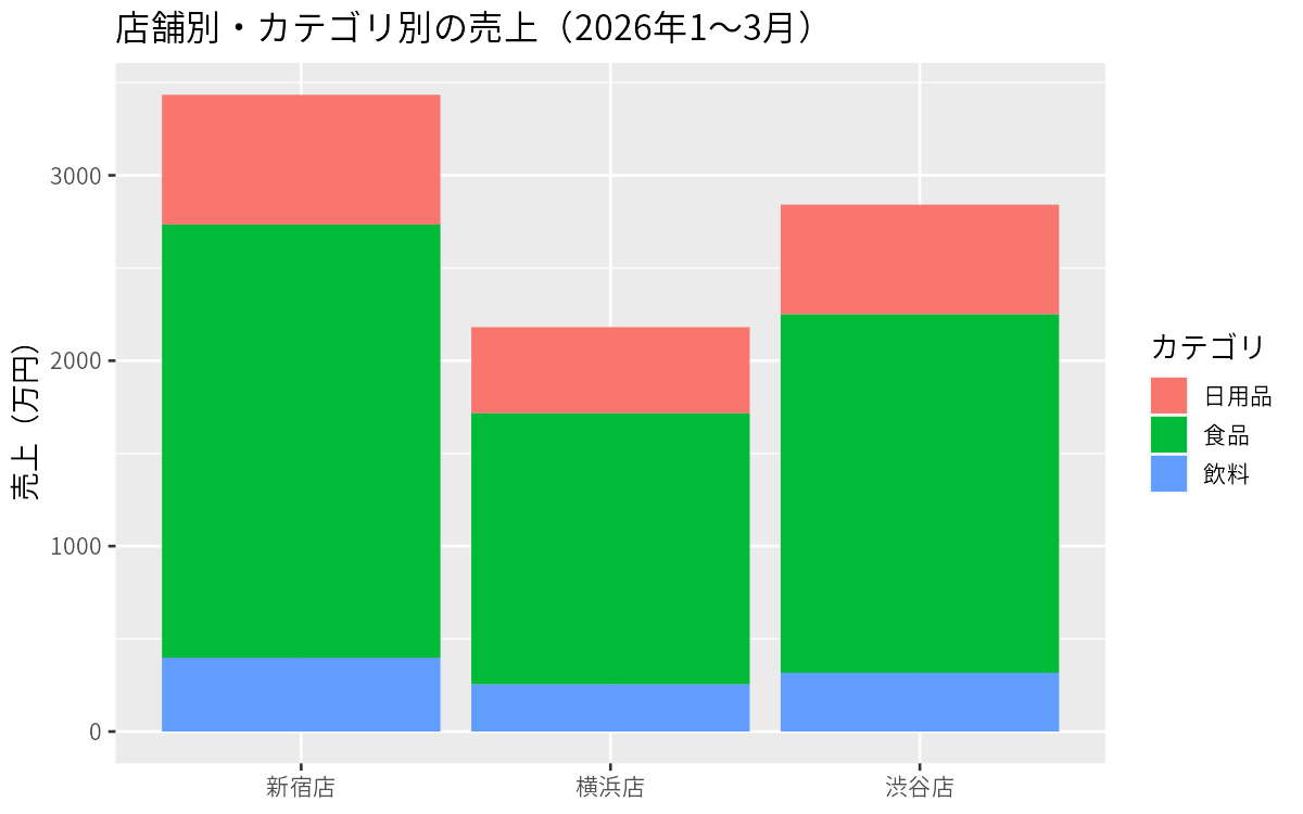
dplyrで集計した結果は、パイプでつないでそのまま ggplot2 のグラフにできます。記事の冒頭の図は、次のコードで作りました。
library(ggplot2)
theme_set(theme_gray(base_family = "Meiryo"))  # 日本語フォント(Macは "Hiragino Sans")

sales %>%
  group_by(store, category) %>%
  summarise(sales = sum(sales)) %>%
  ggplot(aes(x = store, y = sales / 10000, fill = category)) +
  geom_col() +
  labs(title = "店舗別・カテゴリ別の売上(2026年1〜3月)", x = NULL, y = "売上(万円)", fill = "カテゴリ")
グラフの作り方は、次回のggplot2の記事で詳しく解説します。
まとめ
filter()で行、select()で列を絞り込むmutate()で計算した列を追加し、arrange()で並び替えるgroup_by()+summarise()で、ピボットテーブルのような集計ができる%>%でつなぐと、処理の流れを上から順に読める
dplyrを覚えると、Excelで何十分もかかっていた集計が数行のコードで終わり、しかも同じ手順を何度でも再現できます。ぜひ手元のデータで試してみてください。
同じことをGoogle ColabのPythonで行う方法は、pandasでデータ加工入門【絞り込み・列の選択・列の追加・並び替え・グループ集計】で紹介しています。
NEWSLETTER
Data Schoolの新着記事をメールで受け取る
新しい記事が公開されたら、メールでお知らせします。配信はいつでも停止できます。