
Pythonで基本統計量とクロス集計を出す方法【pandasのdescribe・value_counts・crosstab】
 酒井 裕麻株式会社Bistro 代表取締役社長
アンケートや顧客データを受け取ったら、まずやるのが基本統計量とクロス集計です。「平均は?」「年代ごとの購入率は?」といった数字をつかむことで、データの全体像が見えてきます。
この記事では、Google ColabのPython(pandas)で、基本統計量・度数・クロス集計を出す方法を、アンケートデータを使って解説します。
同じことをRで行う方法は、Rで基本統計量とクロス集計を出す方法で紹介しています。
この記事で使うデータ
架空の商品アンケート survey.csv(400人分)を使います。
| 列名 | 内容 |
|---|---|
| id | 回答者ID |
| gender | 性別(男性・女性) |
| age | 年代(20代〜50代) |
| awareness | 商品の認知度(1〜5) |
| price_sat | 価格への満足度(1〜5) |
| ad_contact | 広告を見たか(1:見た、0:見ていない) |
| purchase | 購入したか(1:購入、0:非購入) |
| satisfaction | 総合満足度(0〜10) |
import pandas as pd
survey = pd.read_csv("https://www.bistro.business/files/r/survey.csv")
survey.head()
実行結果
   id gender  age  awareness  price_sat  ad_contact  purchase  satisfaction
0   1     女性  40代          4          3           0         1             6
1   2     女性  50代          3          1           1         0             2
2   3     男性  20代          4          3           1         0             8
3   4     女性  50代          2          2           0         0             4
4   5     女性  40代          5          1           1         0             5
describe()で基本統計量をまとめて出す
describe() を使うと、数値の列の基本統計量を、まとめて出せます。
survey[["awareness", "price_sat", "satisfaction"]].describe().round(2)実行結果
       awareness  price_sat  satisfaction
count     400.00     400.00        400.00
mean        3.15       3.18          6.13
std         1.16       1.05          1.60
min         1.00       1.00          2.00
25%         2.00       2.75          5.00
50%         3.00       3.00          6.00
75%         4.00       4.00          7.00
max 5.00 5.00 10.00| 項目 | 意味 |
|---|---|
| count | データの件数(欠損値を除く) |
| mean | 平均 |
| std | 標準偏差(ばらつきの大きさ) |
| min / max | 最小値 / 最大値 |
| 25% / 50% / 75% | 下から25%・50%(中央値)・75%の位置の値 |
総合満足度は、平均6.13、中央値6で、2〜10点に分布していることがわかります。
平均・中央値・標準偏差を個別に出す
1つの値だけ知りたいときは、それぞれの関数を使います。
s = survey["satisfaction"]
print("平均:", round(s.mean(), 2))
print("中央値:", s.median())
print("標準偏差:", round(s.std(), 2))
実行結果
平均: 6.13
中央値: 6.0
標準偏差: 1.6
value_counts()で度数を数える
文字の列(性別や年代など)は、value_counts() で、それぞれの値が何件あるかを数えます。
survey["age"].value_counts().sort_index()実行結果
age
20代    114
30代    104
40代    105
50代     77
Name: count, dtype: int64
sort_index() で、年代の順に並べています。付けないと、件数の多い順に並びます。
構成比(%)にする
normalize=True を付けると、件数ではなく割合になります。100を掛けて、%にします。
(survey["age"].value_counts(normalize=True).sort_index() * 100).round(1)実行結果
age
20代    28.5
30代    26.0
40代    26.2
50代    19.2
Name: proportion, dtype: float64
クロス集計
2つの項目を掛け合わせる
pd.crosstab() で、2つの項目を掛け合わせたクロス集計表を作れます。性別と、購入したかどうか(0・1)を掛け合わせます。
pd.crosstab(survey["gender"], survey["purchase"])実行結果
purchase    0   1
gender
女性        117  68
男性        137  78
margins=True を付けると、合計の行と列(All)も表示されます。
pd.crosstab(survey["gender"], survey["purchase"], margins=True)実行結果
purchase    0    1  All
gender
女性        117   68  185
男性        137   78  215
All       254  146  400
行ごとの割合(購入率)を出す
性別ごとの購入率を比べるには、行ごとの割合にします。normalize="index" を指定します。
(pd.crosstab(survey["gender"], survey["purchase"], normalize="index") * 100).round(1)実行結果
purchase     0     1
gender
女性        63.2  36.8
男性        63.7  36.3
purchase が1の列が購入率です。女性も男性もほぼ同じで、性別による差はほとんどありませんでした。
| normalize の指定 | 割合の出し方 |
|---|---|
"index" |
行ごとの割合(行の合計が100%) |
"columns" |
列ごとの割合(列の合計が100%) |
"all" または True |
全体に対する割合 |
ラベルを見やすくしたいときは、0・1を「非購入」「購入」に置き換えてから集計します。
label = survey["purchase"].map({0: "非購入", 1: "購入"})
pd.crosstab(survey["age"], label)
実行結果
purchase  購入  非購入
age
20代       47   67
30代       40   64
40代       39   66
50代       20   57
グループごとにまとめて集計する
人数・購入率・平均満足度を、年代ごとに1つの表で出したいときは、groupby() と agg() が便利です。0と1の列は、平均を取るとそのまま「1の割合」になります。
by_age = survey.groupby("age").agg(
    n=("id", "count"),
    purchase_rate=("purchase", "mean"),
    avg_satisfaction=("satisfaction", "mean"),
)
by_age["purchase_rate"] = (by_age["purchase_rate"] * 100).round(1)
by_age["avg_satisfaction"] = by_age["avg_satisfaction"].round(2)
by_age
実行結果
       n  purchase_rate  avg_satisfaction
age
20代  114           41.2              6.27
30代  104           38.5              6.10
40代  105           37.1              6.30
50代   77           26.0              5.75
50代は購入率が低く、ほかの年代より購入につながりにくいことがわかります。
groupby() と agg() の使い方は、pandasでデータ加工入門で詳しく解説しています。
集計結果をグラフにする
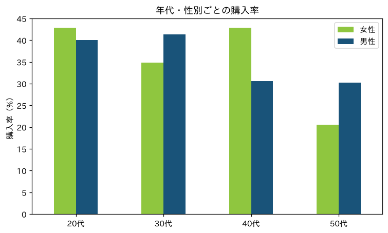
年代×性別の購入率を、棒グラフにしてみましょう。pivot_table() で、年代を行、性別を列にした表を作ると、そのまま .plot() でグラフにできます。
!pip install -q matplotlib-fontjaimport matplotlib.pyplot as plt
import matplotlib_fontja
rate = survey.pivot_table(index="age", columns="gender", values="purchase", aggfunc="mean") * 100
ax = rate.plot(kind="bar", rot=0, color={"女性": "#8FC63F", "男性": "#195379"}, figsize=(8, 4.5))
ax.set_title("年代・性別ごとの購入率")
ax.set_xlabel("")
ax.set_ylabel("購入率(%)")
ax.legend(title="")
plt.show()
まとめ
- 数値の列の基本統計量は
describe() - 文字の列の度数は
value_counts()、構成比はnormalize=True - クロス集計は
pd.crosstab()。行ごとの割合はnormalize="index" - 0・1の列は、平均を取ると「1の割合」になる
- 複数の指標をまとめるなら
groupby()+agg()
集計で差が見つかったら、その差が偶然ではないかを確かめるのが次のステップです。Pythonでt検定とカイ二乗検定をする方法で解説しています。
NEWSLETTER
Data Schoolの新着記事をメールで受け取る
新しい記事が公開されたら、メールでお知らせします。配信はいつでも停止できます。